How large quantum systems can QuTiP handle?

People are often curious to know how many qubits can be simulated on a modern computer, using for example QuTiP. The primary focus of QuTiP is not to manage as large quantum systems as possible, but we do try to make QuTiP efficient, and it is useful to have some feeling for how large systems we can manage.
The answer to the question posed in the title depends strongly on the type of the problem. For example, whether the Hamiltonian is constant or time-dependent, the system is closed or open, states are pure or mixed. Ultimately it is the RAM memory that limits the size of the systems we can manage, but in some cases you are likely to run out of patience long before the RAM memory is exhausted (in particular for time-dependent systems).
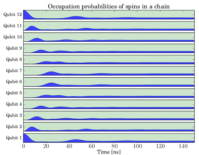
Computationally, the simplest problem that QuTiP will typically be used for is the evolution of a closed quantum system with a constant Hamiltonian. To explore how large quantum systems of this kind we can simulate with QuTiP, let’s consider a chain of spins coupled to their nearest neighbors through a sigma-x interaction. In QuTiP it is easy to program this model in a way that parameterize the number of spins in the chain, allowing us to simulate systems with increasing number of spins until we run out of RAM memory (resulting in a MemoryError exception being raised by python) or until we run out of patience. You can find the program code here:

"""
QuTiP example: Dynamics of a spin-1/2 chain
"""
from qutip import *
from pylab import *
rcParams['text.usetex'] = True
rcParams['font.size'] = 16
rcParams['font.family'] = 'serif'

def system_ops(N, h, J, gamma):

    si = qeye(2); sx = sigmax(); sz = sigmaz()

    sx_list = []; sz_list = []
    for n in range(N):
        op_list = [si for m in range(N)]
        op_list[n] = sx
        sx_list.append(tensor(op_list))
        op_list[n] = sz
        sz_list.append(tensor(op_list))
        
    # construct the hamiltonian
    H = 0
    for n in range(N):
        H += - 0.5 * h[n] * sz_list[n]                # energy splitting terms
    for n in range(N-1):
        H += - 0.5 * J[n] * sx_list[n] * sx_list[n+1] # interaction terms

    # collapse operators for spin dephasing
    c_op_list = []
    for n in range(N):
        if gamma[n] > 0.0:
            c_op_list.append(sqrt(gamma[n]) * sz_list[n])

    # intital state, first and last spin in state |1>, the rest in state |0>
    psi_list = [basis(2,0) for n in range(N-2)]
    psi_list.insert(0, basis(2,1)) # first
    psi_list.append(basis(2,1))    # last
    psi0 = tensor(psi_list)

    return H, c_op_list, sz_list, psi0

def evolve(N, h, J, tlist, gamma, solver):

    H, c_ops, e_ops, psi0 = system_ops(N, h, J, gamma)
    output = solver(H, psi0, tlist, c_ops, e_ops)
    return (1 - array(output.expect))/2.0 # <sigma_z> to excitation prob.

# ---
solver = mesolve              # select solver mesolve or mcsolve
N = 16                        # number of spins
h =  1.0 * 2 * pi * ones(N)   # energy splittings
J = 0.05 * 2 * pi * ones(N)   # coupling
gamma = 0.0 * ones(N)         # dephasing rate
tlist = linspace(0, 150, 150)

sn_expt = evolve(N, h, J, tlist, gamma, solver)

# plot excitation probabilities for each spin
yvals = []
ylabels = []
for n in range(N):
    x = 0.1 # spacing between stacked plots
    p = real(sn_expt[n]) * (1-2*x)
    base = n + zeros(shape(p)) + 0.5 + x
    plot(tlist, base, 'k', lw=1)        
    plot(tlist, base+(1-2*x), 'k', lw=1)        
    fill_between(tlist, base, base + p, color='b', alpha=0.75) 
    fill_between(tlist, base + p, base + (1-2*x), color='g', alpha=0.2)
    yvals.append(n + 1)
    ylabels.append("Qubit %d" % (n+1,))

autoscale(tight=True)
xlabel(r'Time [ns]',fontsize=14)
title(r'Occupation probabilities of spins in a chain', fontsize=16)
yticks(yvals, ylabels, fontsize=12)
savefig('spinchain-%d.pdf' % N)

In this simulation, we initially put excitations at the spins at the end of the chain and evolve the state vector. The result shows how the excitations propagate in the spin chain and eventually disperse.

My patience ran out after 21 spins. This corresponds to a very large quantum state space, 2’097’152 states to be exact, which is a quite impressive number. But admittedly, this simulation took a long time to run: About 7 hours on my laptop, and the memory usage peaked at about 4.3 Gb of RAM.
Open quantum systems are significantly more computationally demanding to evolve. First, we need to use the density matrix rather than a state vector to describe the system, which immediately squares the problem size. Second, the equations of motion (Master equation) are more complicated, including for example superoperators, requiring us to rearrange the equations of motion to obtain an ODE on standard form (of squared system size). Alternatively, we can use a stochastic equation of motion, such as the quantum trajectory Monte-Carlo method, and circumvent the requirement to square the system size, but this also comes at a steep price as we then need to average a large number of trajectories with the original system size. Regardless if we use a master equation or the Monte-Carlo quantum trajectory method, we cannot hope to evolve as large systems as we could for a closed quantum system.

Including dissipation in the example program above (by selecting gamma=0.0025), I could simulate systems up to 12 spins before the RAM memory was exhausted (on a 16Gb desktop). The 12 spin simulation took a weekend to run, and the peak memory usage was about 20 Gb (temporarily swapping 4 Gb). On this computer, further increasing the system size would result in memory error when using the master equation solver. Using the Monto-Carlo solver (by setting solver=mcsolve in the code) I could simulate open systems up to 16 spins in a similar time period (a few days).
If we include a time-dependence in for example the Hamiltonian, the memory foot-print is not significantly altered, but the problem becomes more CPU demanding, increasing the simulation time by sometimes quite a lot. However, at least in principle, we can simulate time-dependent quantum systems of similar size as time-independent problems.